TimeSeries with Python _ Holt-Winters _ Prediction(Foresasting) _ Python

 이번 포스팅에서는 지난번에 다루었던 Holt-Winters Method를 이용해 train 기간 데이터에서 파라미터들을 추정하고, 추정한 파라미터들을 이용해서 예측값을 알아보고 실제값과 비교를 해보는 내용을 포스팅 하겠다.

 

실제 TimeSeries 뿐만 아니라 딥러닝에서도 Train Periods에서 파라미터들을 설정하고 그것들을 이용해 예측을 한 후, Test Periods에서의 실제값과 비교를 하는데, 많이 사용되는 방식이며 비슷한 흐름들이기 때문에 파이썬으로 Forecasting을 하는 방식들이 이와 유사하다고 생각하면 될 것 같다.

df = pd.read_csv(path, index_col = 'Month', parse_dates=True)
df.index.freq = 'MS'
df.head()
df.info()

#%% Train 및 Test 기간 나누기

train_data = df.iloc[:108] # iloc의 경우 인덱스 번호 기준으로 지정을 하는거고, 만약 Date로 할 경우 df.loc[:'2012-01-01']으로 지정
test_data = df.iloc[108:]

#%% Fitting Parameters

from statsmodels.tsa.holtwinters import ExponentialSmoothing

fitted_model = ExponentialSmoothing(train_data['Thousands of Passengers'], trend='mul',seasonal='mul',seasonal_periods=12).fit()

#%% Forecasting

test_predictions = fitted_model.forecast(36).rename('HW Forecast')

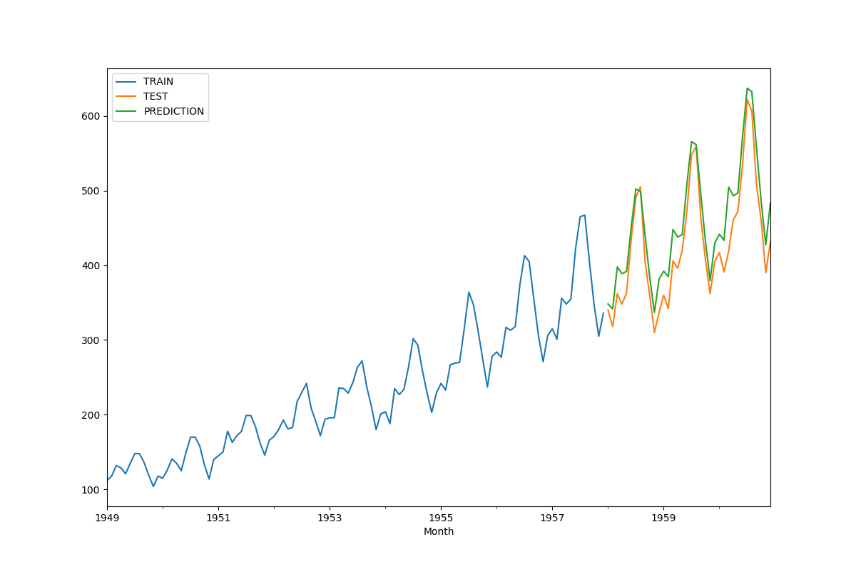
train_data['Thousands of Passengers'].plot(legend=True,label='TRAIN')
test_data['Thousands of Passengers'].plot(legend=True,label='TEST',figsize=(12,8))
test_predictions.plot(legend=True,label='PREDICTION')

#%%

train_data['Thousands of Passengers'].plot(legend=True,label='TRAIN')
test_data['Thousands of Passengers'].plot(legend=True,label='TEST',figsize=(12,8))
test_predictions.plot(legend=True,label='PREDICTION',xlim=['1958-01-01','1961-01-01'])

데이터 전체기간의 Train, Test, Prediction을 살펴본 경우

Predicion과 Test를 살펴본 경우